Simulations in economics

Contents

• 1. Introduction
• 2. Recap
• 3. Applications
• 4. Discussion
• 5. Conclusion

1. Introduction

Simulation, as a research approach in economics, is not as popular as analytical, empirical, or experimental methods. This article provides an expository summary of the simulation as a research tool, its strengths and weaknesses, and how it can be used in economic research.

2. Recap

First of all, let’s recap the various approaches in economic research. Analytical approach tries to find a mathematical formulation of a phenomenon to understand and/or predict it. Empirical approach uses real-world data to explore the phenomenon. The following example illustrates the difference.

2 a. Chessboard example

Imagine a chessboard with a king on the cell a1. Every minute, the king moves one cell up and one cell right. What will be the location of the king after 5 minutes?

• Analytical solution identifies that at minute t, the king is on the cell denoted by t‘th letter of the alphabet and number t:

Plugging in t=1+5=6 into the equation gives the location of the king after 5 minutes as f6.

• Empirical solution observes the king for the first 3 minutes and extrapolates a pattern.

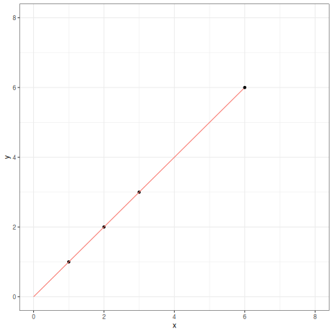
Fitting the curve, it forecasts the location of the king after 5 minutes as f6.

• Simulation, on the other hand, does not make any assumptions or estimations — it takes the initial location parameter a1 and the update rule “1-up-1-right” and runs it in a computer for 5 periods as follows:

The advantage of simulations becomes clearer when we consider more complex problems. Imagine a chessboard with the following pieces and movement rules:

1. white king on a1: moves 1-up if it is on a black cell and 1-right if it is on a white cell
2. black bishop on c8: moves 1-right-1-down
3. white knight on h1: moves 2-left-1-down if it is on a black cell and 2-up-1-left if it is on a white cell
4. black bishop on f8: moves 1-left-1-down
5. capture is required if possible
6. each piece performs one move per period

What is the state of the chessboard after 3 periods?

Analytical model gets complicated even at this very simplified special case of a chess game. Empirical models can help only in presence of the relevant data. Simulation comes handy in this type of problems because it does not look for a solution or estimation — it simply runs the game and sees what happens. In fact, this is how chess engines work.

A similar example is Rubik’s cube — it is possible to provide an analytical explanation of what a 3-move combination does, but it is very difficult to grasp what a 12-move combination does — that’s why the usual way to understand the combinations is by starting from a completed cube and actually performing the moves and seeing the results after the fact, which is exactly what simulation does. Let’s take a look at another example, this time from economics.

2 b. One-time investment

Imagine a stylized scenario, when you are 25 years old and have 1,000$ and want to make a one-time investment for your retirement at 65. You have two options: invest immediately at 5% annual interest rate or invest at age of 35 at 7% annual interest rate. In the absence of discounting and any kind of time preference, which investment will you choose?

• Analytical solution uses a compound interest rate formula to compare the values:

• Empirical approach surveys 100 people who invested in either option and asks their wealth at retirement.
• Simulation codes a program, where two hypothetical scenarios take place and compares the results:

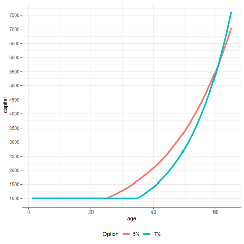
Simulation focuses on the evolution of portfolio through time as much as it focuses on its value at retirement. In the above example we can see that the first investment option is better until 60 years and worse after age 60. However, the real advantage of using simulations can be realized when analyzing a more realistic situation, when you make investment contributions every month of your life and the portfolio values change with the economy and stock markets. In this situation, analytical solution gets extremely complicated, and the portfolio choice is better analyzed using simulations. Below is one example of how simulations make life-cycle investment analysis easier in case of multiple stocks changing at the same time.

2 c. Confidence interval

Consider two random variables A and B. A is normally distributed around 5 with standard deviation 10, and B is normally distributed around 3 with standard deviation 5. What is the confidence interval of A+B?

We can get into joint distributions or use theorems to solve the problem, but there is another way — to perform a simulation with 10,000 scenarios, where in each scenario we draw values from the distributions of A and B and sum them:

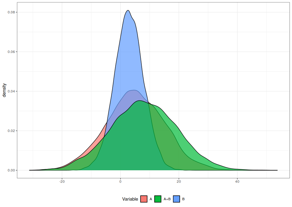
Using simulations, we have obtained a new variable A+B with one mean and one variance instead of original two. Thus, we can calculate the confidence interval from the resulting data, without having to use multivariate probability theory. The advantage becomes clearer when we want products or other nonlinear combinations of the two random variables.

The examples above illustrate two important characteristics of simulations: (a) they allow us to study not only the results, but also the evolution of states leading to the results, and (b) they allow for higher complexity in problem formulations. The latter comes from the fact that simulations do not require a solution, and simply implement the process given the initial parameters and the rules. Before we proceed to the discussion of the methodology, let’s take a look at the actual research that employs simulations.

3. Applications

Reading the previous section might give a false impression of a strict choice among different research tools. However, actual simulation studies heavily involve both analytical and empirical aspects, as can be seen below.

3 a. Portfolio selection

An individual wants to choose among different life-cycle investment strategies for the retirement. The decision is to allocate funds to stocks and bonds. The candidates are listed below:

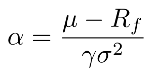
1) Markowitz : a classical investment rule in financial economics — to invest the following percentage of the funds in stocks (and the rest in bonds):

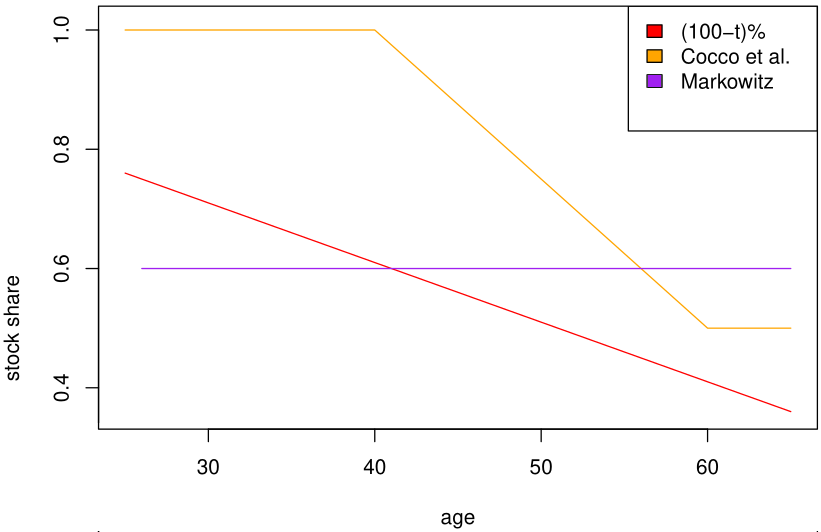
2) α=(100-age)% : invest (100 - age)% of the funds in stocks, and the rest of funds in bonds — this has been a usual (empirically obtained) advice by financial consultants of the second half of the 20th century.

3) Cocco et al. : an upgrade to the previous rule — a rule to invest the following ratio of funds in stocks:

where t is age of an investor. This heuristic has been obtained from series of dynamic optimizations (speaking of analytical aspects of a simulation study).

The following graph illustrates the ratio of funds to be invested in stocks for different ages:

The law of motion of the capital follows the following dynamic:

where w_t is the wage of the individual at time t, c is the portion of the wage allocated for investment, and r_p is the rate of return of the portfolio of choice.

Regardless of the portfolio choice, the following processes happen in the background: wages change throughout lifetime (at different rates for different individuals), stock prices change depending on an economic situation.

Moreover, calculating the final capital is not enough for a comprehensive comparison — we have to take into account the individual characteristics like risk aversion, steepness of the earnings curve, and the industry at which the individual works.

This model contains too many moving parts to try to solve it analytically. Even the calculation of the confidence intervals is very difficult, because there are at least two sources of randomness — labor markets and stock markets. And we didn’t even include housing investment!

Simulation is very useful for this type of problems. We can approach the solution as follows:

1. Consider a 25-year-old agent that wants to invest in a pension fund.
2. Randomly generate prices for all assets in a portfolio for the whole investment timespan (40 years in this example) from the given distributions (calibrated from the historical data).
3. Calculate portfolio values according to the generated state.
4. Let the agent invest in 3 portfolios and observe the funds until age 65.
5. Repeat the above steps N=10,000 times.

The resulting data can be used to test different insights — from observing mean and variation across scenarios to comparing the relative frequency of preferences. Below we present just one of the possible results of the simulation — how frequent one portfolio is better than the other:

As you can see, simulations work really well for comparing different scenarios, as the values themselves are not informative.

3 b. Prisoner’s Dilemma

Simulations also come in handy for observing the behavior of agents in game theoretic contexts. Consider a standard Prisoner’s dilemma with two agents and the following payoff matrix:

We can model a so-called agent-based simulation where each agent decides to deviate or not, and, sure enough, they converge in a Nash equilibrium:

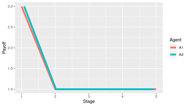
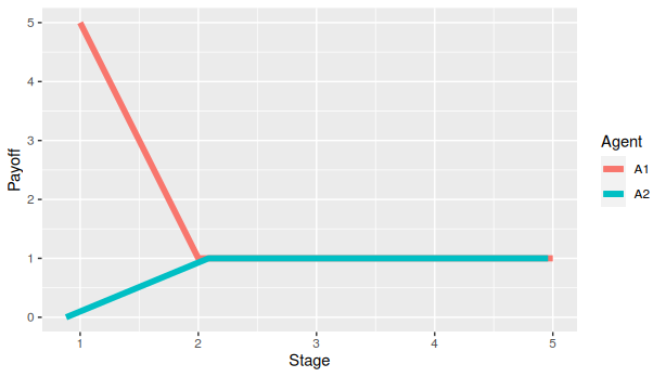
As mentioned above, you can see the advantages of the simulation when the problem gets more complicated, e.g. multi-player Prisoner’s dilemma. An even more interesting application can be to play with the behavioral stuff. For example, we can simulate a repeated game, however the agents are bounded-rational, i.e. they can only see a few periods in the future — this can help to find new insights and new equilibria.

4. Discussion

As we can see, simulations are more than just data-generating tools and can be used for more ambitious applications.

At the same time, however, we have to be careful not to rely on it unconditionally, because every finding from simulations is determined by the structure and the input parameters we set ourselves.

That is one of the reasons, why simulations work better for comparative dynamics rather than absolute analyses: we can transform, modify and normalize our obtained datasets, and this will still be valid for comparing scenarios.

Another implication is that, by definition, the only surprising findings from the simulations should be due to complexity. Any unexpected results from simpler models are highly likely to be caused by the error in formulation or code. On the bright side, you can validate your model for simpler cases and then make the model as complex as you want, and your only limitation will be your computing power, and not the theoretical solvability.

Moreover, we have to be aware that simulation-generated data always loses to the real-world data, and that is why we can see the surge of simulations research when a new phenomenon happens and no data is available, which was exactly what happened with COVID-19 research.

Another interesting question is why do the video games have the economy building / country managing capabilities for two decades, and economics simulation does not. The answer is that for video games you only need the economy structure and parameters hard coded, and the outcome is randomly generated. However, for the research, you have to control for all variability and repeat simulation for a few thousand times, this is what uses the most computational power, memory, and time. And this is what makes simulations research lag behind video games simulations.

5. Conclusion

In this article I tried to make a non-intrusive introduction to the simulations as a research tool (as opposed to an auxilliary data-generating tool). I have presented a few examples and discussed the weaknesses of the approach that I had discovered from my two years of experience in the field. For questions, please do not hesitate to contact me.