My take on the famous medical appointment no-show problem

Contents

• 1. Introduction
• 2. Data exploration
• 3. Classifier
• 4. Conclusion

1. Introduction

This is a famous problem from Kaggle website. We have a dataset of online medical appointments in the city of Vitória, Espírito Santo in Brazil. It turns out that in a period of three months between May and August, 2016, patients did not show up in 25% of appointments. To investigate the possible reasons behind this, we will analyze the data and make inferences.

2. Data exploration

Outliers

First of all, we explore the dataset. We immediately notice that some age values are negative, and very old patients don’t exhibit variation having too few observations:

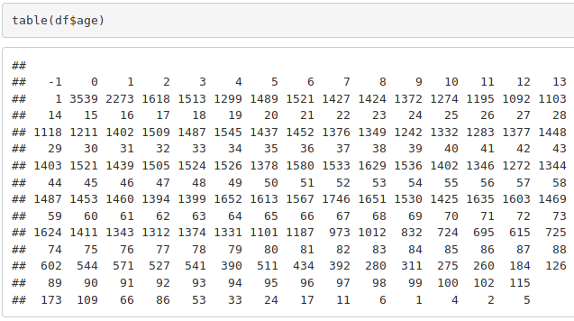
Moreover, some appointments have been done to the dates before it was scheduled, probably, due to some system error. We remove the obvious outliers from our data, combine all data points for households older than 80 (to balance subset size), and continue with our analysis.

df <- df[ (df$age >= 0) & (df$dayap >= df$daysc),]

Demographic factors

Age factor

Observing the no-show dynamics throughout lifetime, gives important insights to our analysis:

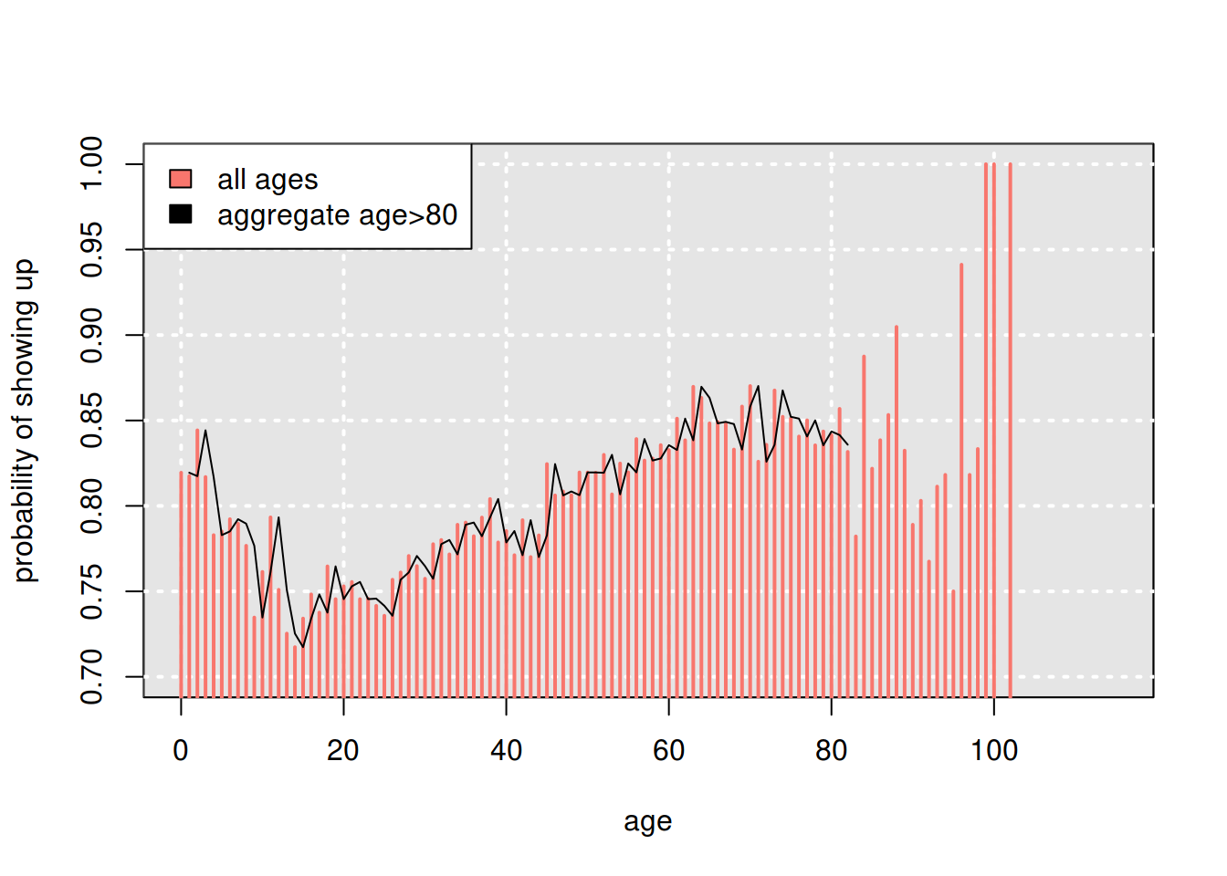
From common experience, we know that appointments for patients younger than 18, are actually done by their parents. We can see how, as kids grow older, the parents tend to miss more appointments (because new parents tend to be concerned more with infant’s health, and as kids grow, parents tend to neglect their health slightly more).

As kids grow into young adults, they start steadily taking their health seriously and miss less appointments.

Also, for patients older than 80, we don’t have many data points at particular ages, so we aggregated them into one group.

So, we use two possible age variables: a continuous one with two dummies for 18 and 80 year olds, and a discrete variable correpsonding to 11 decades of patients.

Gender factor

Another demographic factor is gender. The probability distribution shows that gender does not play a significant role in no-show rate:

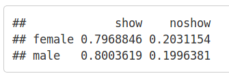
We tried to look at adults only (age>=18), because usually mothers (female=1) go to doctors with their children, irrespective of the kid’s registered gender, but this procedure returned no significant difference either:

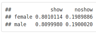
Thus, we ignore gender in further discussion.

Geographic factor

Looking at no-show rates by neighbourhood, shows relative balance, with only a few outliers, which do not round to 20\%.

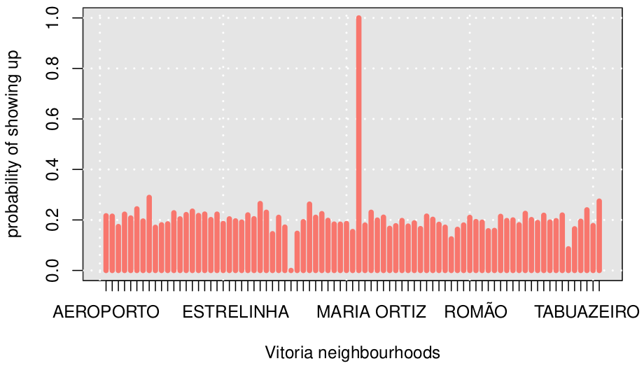
Inspecting frequency tables, shows that most (not all) of the outliers come from neighbourhoods with little data:

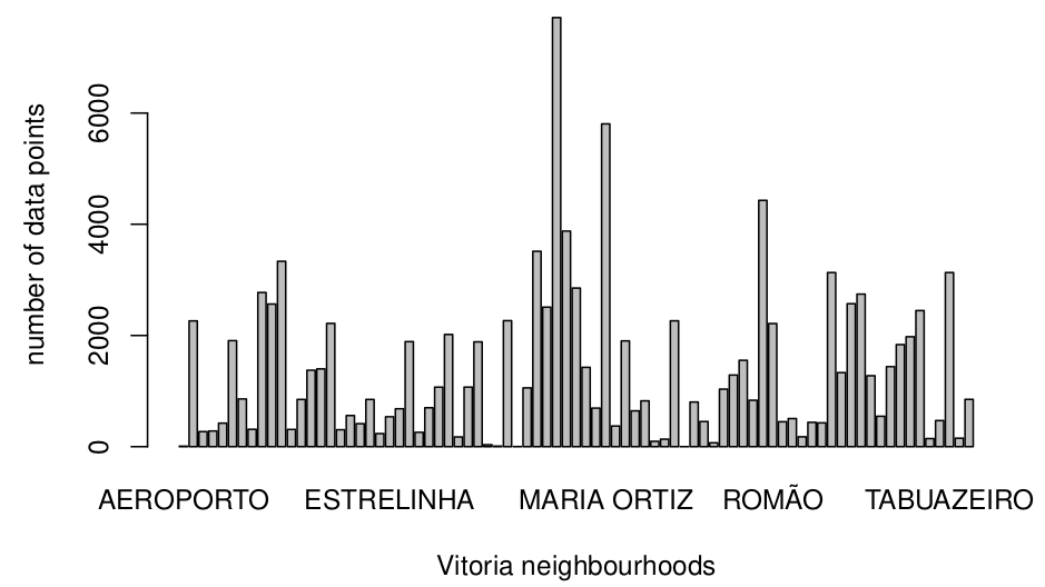
To avoid this, we ignore neighbourhoods with less than 40 data points, namely, Aeroporto, Ilha do Boi, Ilha do Frade, Ilhas Oceanicas de Trinade, and Parque Industrial.

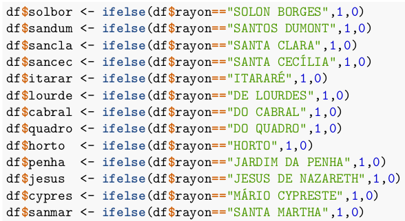
Apart from them, there are still outliers (we considered 3% to be a significant deviation from the average, 20%) in percentage of no-shows: Solon Borges, Santos Dumont, Santa Clara, Santa Cecilia, Itarare, De Lourdes, Do Cabral, Do Quadro, Horto, Jardim Da Penha, Jesus de Nazareth, Mario Cypreste, and Santa Martha.

We will add dummy variables for these 13 neighbourhoods as our geographic predictors. Other neighborhoods will be assumed to contribute no new information to the expected value.

Temporal factor

Temporal data brings the crucial information about the appointment no-shows, starting from the weekday of the appointment, and ending with the wait time. Since we don’t have at least a year-long data, we cannot speak of seasonality patterns, and will have to get by with what we have.

Weekdays

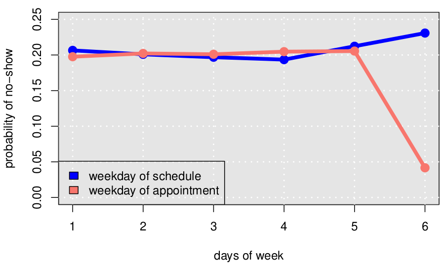
The day of the week is the first thing that comes to mind - during the weekdays, patients might have emergencies at school or at work, and this could cause them to miss the appointment. However, the analysis shows no significant difference through week, except for Saturdays:

But further analysis shows that this happens because of the lack of enough data for Saturday:

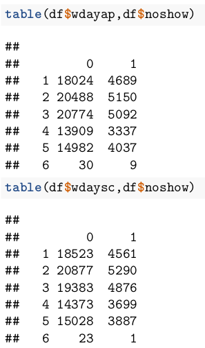
So, we ignore the weekdays and assume that they don’t affect the no-show rate.

Wait time

Another obvious variable is a wait time from scheduling the appointment to the appointment itself. It is plausible to assume that in longer wait times patients can get cured, book another earlier appointment, or die before the appointment.

We define the “days between” variable as the difference between “day of appointment” and “day of schedule”:

df$daybw <- as.numeric(df$dayap - df$daysc)

The plot below shows that when appointments are scheduled in that same day (wait time = 0), the patient almost never misses it (just 4\% no-show rate). There is sufficient data (34\% of all observations) to support this claim.

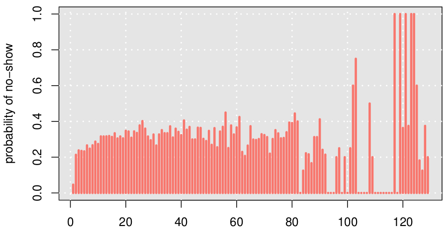
In the next days, the no-show rate is very volatile. To avoid weekly seasonality, we aggregate the data by weeks. Also, for two reasons: (i) since the longer wait times have small data points and (ii) since (assuming time discounting — a weak economic assumption) people perceive recent past clearer than distant past, we aggregated first month as 4 weeks, and aggregated the next data points by month:

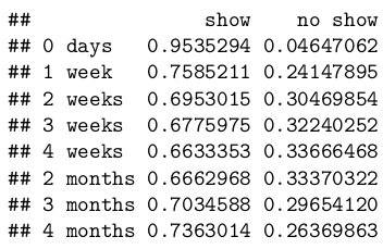
Note that 4 months wait is an outlier due to small dataset. Otherwise, all probabilities after 1 week fall into ±3\% interval. Taking this and (ii) into consideration, suggests an even wilder (yet still plausible) aggregation: 0 days, 1 week, and >1 week:

Thus, we will use three-valued categorical variables to denote wait times.

Hour of the day

Lifestyle of people potentially reflects their degree of responsibility — “night owls” tend to sleep during days and maybe miss deadlines, while “early birds” may take their appointments more seriously. We take a look at the data of time o’clock when the appointment was scheduled. The online appointment system opens at 6AM and closes at 10PM. We divide these 16-hour days into 4 groups of 4, and find that “early bird effect” actually exists, and people who scheduled appointments between 6AM and 10AM are significantly less likely to miss their appointments, while any other time slot does not change the no-show probability significantly:

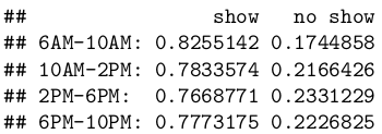
Thus, we use a binary dummy variable — 6AM-10AM or 10AM-10PM — to incorporate time.

Medical factor

Appointment history

To incorporate the idiosyncracies of patients, we use the history of their previous appointments, and whether they missed them before. The table below shows the repeat patients’ allocation.

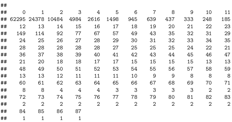
For every patient, we found the modes (most frequent observations) of previous no-show stats. For patients that appear in the dataset only once, this value will be 0 (performing sensitivity checks we learned that leaving out one-time patients entirely, returns no significant difference (<0.5%) but complicates the dataset, so we chose to set the average previous no-show rate for first-time patients at 0). We observe that such modes greatly contribute to predicting the next no-show:

Patient condition

Patient’s medical history can influence the no-show behavior. The tables below show differences in percentage of no-shows for patients with alcoholism, diabetes, hipertension, medical financial assitance (so-called “scholarship”), and handicaps:

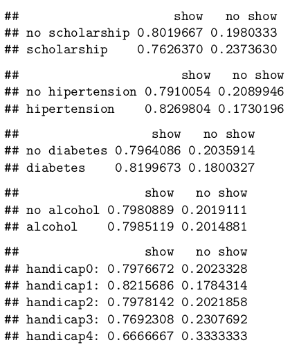
Strangely, alcoholism is the only condition which turned out to not have an effect on no-show probability. The probable reason is that alcoholism is not immediately lethal, and people tend to treat is less seriously than any other “more serious” illness like diabetes. So, we include all of the above conditions, except alcoholism, in our classification.

SMS

One can justifiably argue that patients may simply forget their appointment date and time. Hospitals tried to send SMS-reminders to their patients, but does this practice worth the cost? A simple frequency table shows that yes, patients, who received SMS-reminders, were less likely to miss the appointment:

Overall no-show stata

Finally, we decided to include the general historical average of noshows till the moment by all patients. However, this complicated the random sampling, and, most importantly, didn’t affect the final result much (because it had little variation over time). So, we did not include this variable.

3. CLassifier

We used logit (logistic regression) and decision trees to classify the data.

Logit

df$waittime <- ifelse(df$daybw==0,0,ifelse(df$daybw<=7,1,2))
df$morning <- ifelse(df$hoursc>=6 & df$hoursc<=10, 1, 0)
df$age18 <- ifelse(df$age>=18,1,0)
df$age80 <- ifelse(df$age>=80,1,0)
df$age_decade <- floor(df$age/10)
trainsize <- round(nrow(df)*0.8)
dftrain <- df[1:trainsize,]
dftest <- df[(trainsize+1):nrow(df),]

logit <- glm(formula = 
               noshow ~ age + age18 + age80 +
               burs + diabet + handcap + alcohol +
               solbor + sandum + itarar + lourde + cabral + quadro + penha + jesus + sanmar +
               sms + morning + waittime + mode_previous,
             family = binomial(link="logit"),
             data = dftrain
             )
summary(logit)

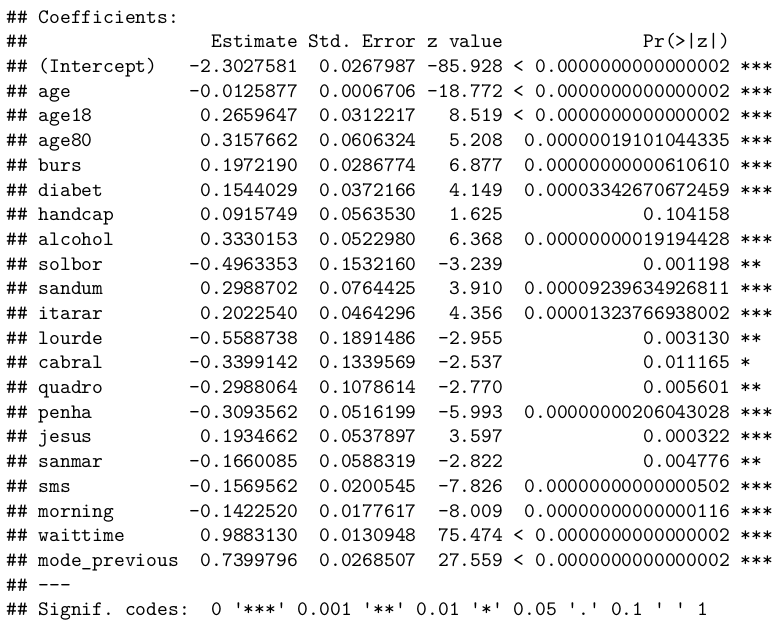
We found that the wait time, previous no-show history, and geographical location were the most important predictors. Also, alcohol turned out to be statistically significant, while hipertension had to be removed from the final model. Strangely, eligibility to financial assistance increased the likelihood of no-show (but this was discussed in the previous section).

To check the accuracy of the model, we predict the no-show for the test data and use measures called accuracy and AUR:

predicted_noshow <- ifelse(predict(logit, dftest,type = "response")>=0.5,1,0)
actual_noshow <- dftest$noshow
mytab <- table(abs(predicted_noshow - actual_noshow))

accuracy <- mytab[1]/(mytab[1] + mytab[2])
accuracy
roc(actual_noshow, predicted_noshow)

So, we have 81\% accuracy, but this is not a very desirable result because of data imbalance — if we just set all “noshows” to zero, we would still get 80% accuracy. The measure AUR confirms this by giving the result 52.9\% — which is slightly better than saying “fifty-fify”.

So, we decide to take a look at decision trees:

Decision trees

Before doing the decision trees, we will undersample our majority set (noshow==0). The resulting tree returns 60\% accuracy and 69\% AUR on average. Different tree specifications give different resulting trees, but the average accuracy doesn’t change. The recall is 80\% on average, though. Here is just one of the trees. Notice that we used age as decades here, and not as a continuous variable:

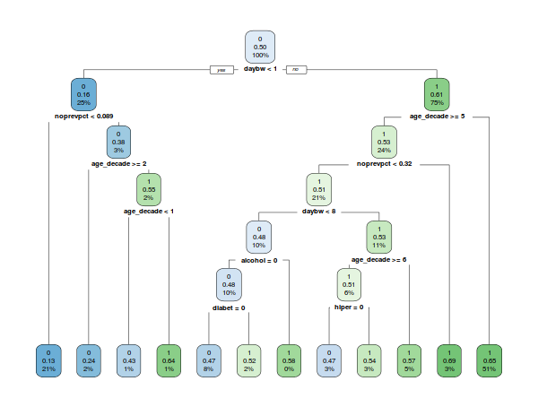
The above tree is not the one I ended up using, the other ones just didn’t fit the page.

4. Conclusion

We have analyzed the data and tried to do a classification analysis. The results are not perfectly accurate, but they are not worse than a naive “noshow=0” prediction.

As an economist, I believe that having a higher accuracy would be impossible without additional data, like weather that day (was it rainy or not), the traffic situation, the diagnosis, the local news etc.

You can see my code in the following repo: github.com/ravshansk/kaggle.

I believe my approach is wrong in many ways, so I welcome your feedback.